MATLAB-SIMULINK TUTORIAL for ECHE 550
This
tutorial can be found on the web at:
http://opus.che.sc.edu/~gatzke/courses/tutorial.htm
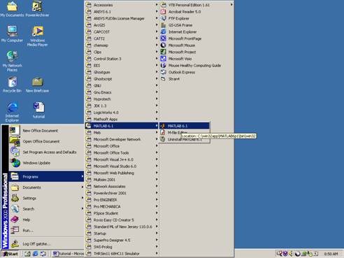
1.
From the “Start”
Menu in the lower right corner, start MATLAB.

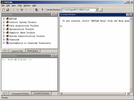
2.
You should get
the following PC Matlab window:
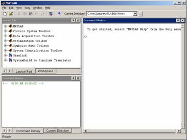
3.
At the command
prompt in the “Command Window” enter the following command:
>> simulink
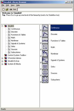
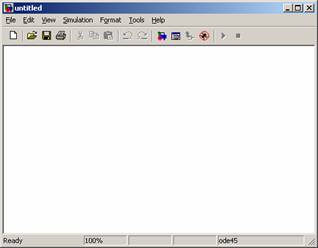
4.
From the “File”
menu select “New” then “Model”
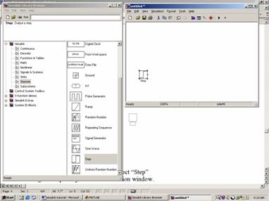
5.
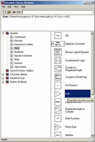
In the Simulink Library Browser window, click (or double-click) on
“Sources”.
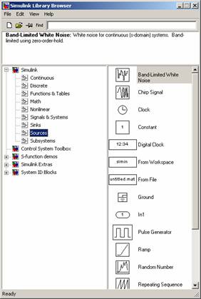
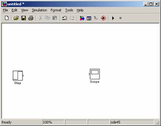
6.
From the bottom
of the list of blocks, select “Step” and drag the step into your blank
simulation window.
7.
In the Simulink Library Browser window, click (or double-click) on
“Sinks”.
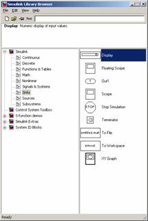
8.
Select a “Scope”
block and drag it into your untitled Simulink
simulation window.
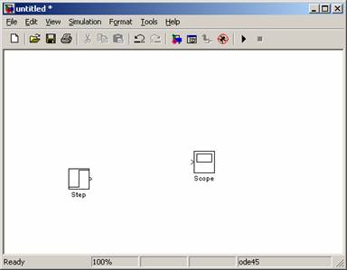
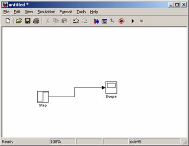
9.
Select the arrow
coming out of the Step block and connect it to the arrow going into the scope
block.
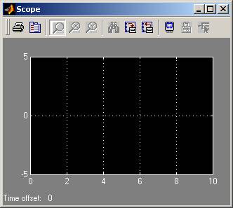
10. Double click on the Scope block to open a scope
window:
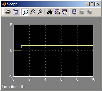
11. To start your simulation running, in your untitled
simulation window hit the play button (top, second from right). Note that you can also select
“Simulation->Start” using the menus of the simulation window. You should see the following in your scope
window:
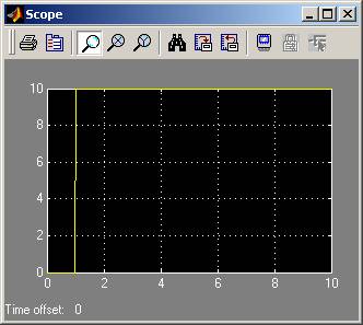
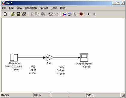
12. In your untitled simulation window, double click on
the step block. Change the “Final Value”
to 10 and run the simulation again. Your
scope should look like:

13. Hit the binocular button, and the axes will
rescale:
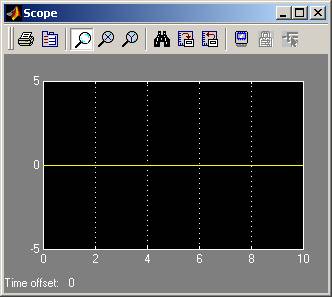
14. In the untitled simulation window, double click on the
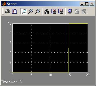
step block and change the step time to 15, then run the simulation. Your scope should look like:
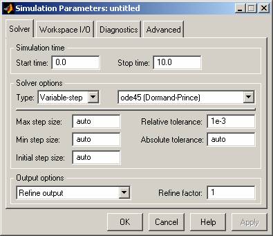
15. You did not run the simulation far enough in
time. In the untitled simulation window,
select from the “Simulation” menu “Simulation Parameters”. Change the stop time to 20.
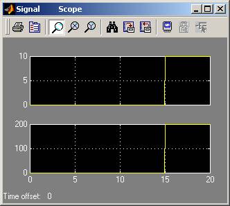
16. Run the simulation, hit the binocular button, and your
scope should look like:
17. To lock this axis value (so you don’t have to hit the
binoculars each time, hit the button to the right of the binocular button.
18. You should now save your untitled simulation. From the “File” menu in the untitled
simulation window, select “Save”. You
can save your file in your Z drive (H:) so that it
will be accessible from any of the engineering PCs.
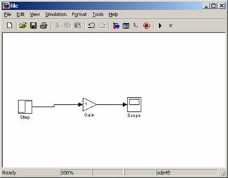
19. Now, we will modify the simulation slightly. Select the connection between the step block
and the scope in your simulation window, and hit delete:
20. In the Simulink Library
Window, click on “Math” and select a Gain block:
21. Drag the Gain into your simulation window and connect
the simulation as follows:
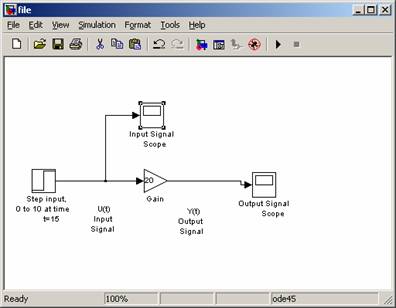
22. Double click on the Gain block in you simulation
window and change the value of the gain from 1 to 20. Run the simulation, then hit the binocular
button on the scope window:

23. We need to label our simulation. You can double click
on the background of your simulation to enter text:
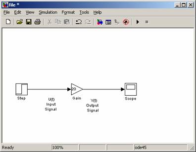
24. You can also edit the text for each block, to make the
simulation more descriptive.
25. We would like to look at the input signal and the
output signal. Click on the Scope block
in your simulation, then select copy (Edit Menu-> Copy or Control-C or the Copy
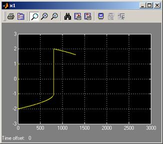
button). Hit paste (Edit Menu ->
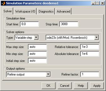
Paste or Control-V or the Paste button).
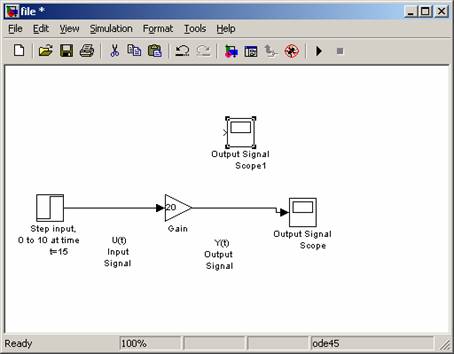
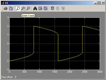
26. From the new scope, select the input arrow, and drag
the line to connect to the signal between the step and the gain. When you are lined up properly, the
crosshairs turn from single to double, then release
the mouse.
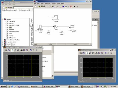
27. Now open both scopes, run the simulation, and hit the
binocular buttons on each scope:
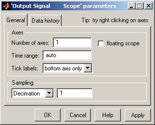
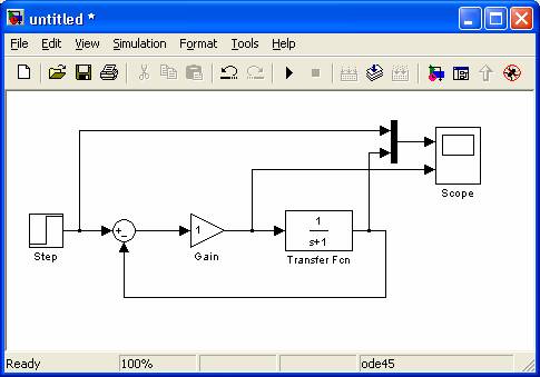
28. Instead of having two scope windows, you can have two
axes in one scope. Select your output
scope window and hit the second button from the left, the “Parameters” button. Change the Number of axes from 1 to 2 and hit
“ok”:
29. Delete your input scope, then modify your simulation
so that the input signal and the output signal are fed into the scope:
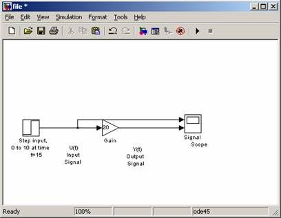
30. Run the simulation.
31. Change the name on your scope block in the Simulink window to uniquely identify yourself. This will cause the title of the scope to
change to your name. Run the simulation and print out your scope
and your simulation window to hand in.
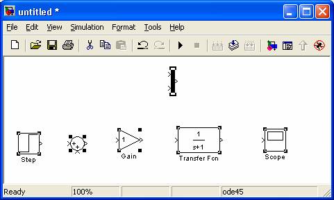
32. Create a new blank simulation. You will need
a.
a step (From
“Sources”)
b.
a scope (From
“Sinks”)
c.
a sum block (From
“Math”)
d.
a gain block
(From “Math”)
e.
a transfer
function block (From “Continuous”)
f.
a mux block (From “Signal Routing”) Your simulation window should look like:
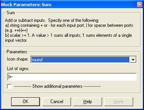
33. Double click on the Sum block and change the value
from “|++” to “|+-“ .
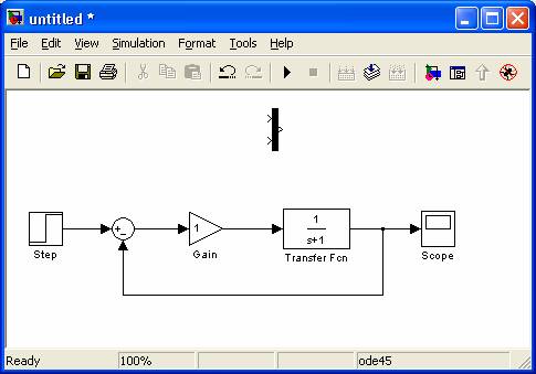
34. Now, you are going to create your first feedback
control system. The transfer function
represents a simple linear dynamic system relating process input u(t) to process output y(t).
The gain block is a simple controller.
The step is a change in ysp(t). The sum block
calculates the error between ysp(t) and y(t). Connect
your blocks in the following manner:
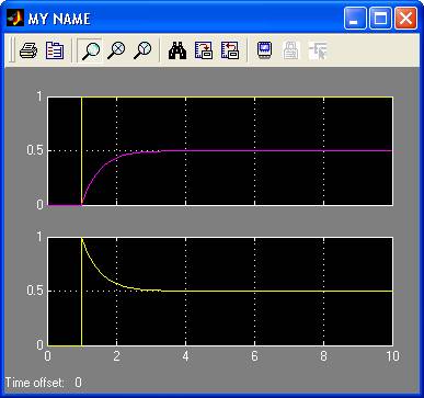
35. Run the simulation and look at the response. You should see a response that starts at
zero, and starts gradually changing toward 0.5 at time t=1.0.
36. Now, change the scope block to accept two input
signals. Connect your blocks in the
following manner:
37. Change the name of your scope block to identify
yourself when you print it out.
38. Select in your simulation window, “Format” -> “Wide
Nonscalar Lines”.
Also select “Format” -> “Show Port Widths”. Simulink can accept
vector values for some blocks. Your
simulation window should look like: 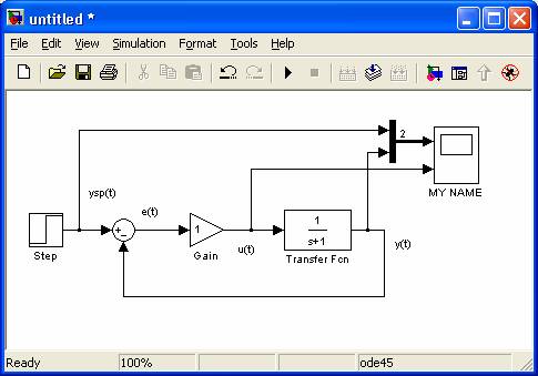
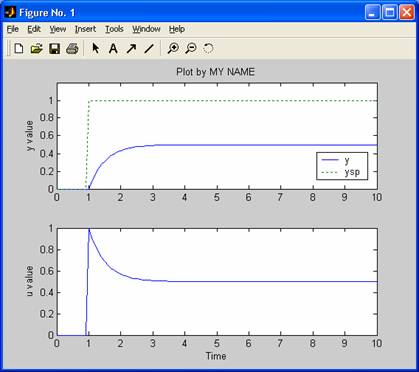
39. Run the simulation, and print out your response to turn in. The top graph shows the setpoint and process measurement on the same plot. The bottom graph shows the input move
calculated by the simple control system.
40. Now, add a clock block from “Sources” and a “To
Workspace” block from sinks. Click on
the “To Workspace” block and change the sample time to 0.1, select save format
as “array” and change the variable name to “t”.
41. Copy / past the “To Workspace” block
three times, and change the variable names to “y” “ysp”
and “u”.
42. Connect your blocks in the following manner: 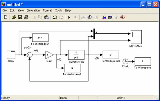
43. Run the simulation.
In the matlab window, type “whos”. You should
see something like:
>> whos
Name Size Bytes Class
t 101x1 808 double array
tout 103x1 824 double array
u 101x1 808 double array
y 101x1 808 double array
ysp 101x1 808
double array
Grand total is 507 elements using 4056 bytes
>>
44. Type “edit” in the matlab
simulation. An editor window should
appear.
45. Type in the following commands:
subplot(2,1,1)
plot(t,y,t,ysp,':')
legend('y','ysp')
ylabel('y value')
title('Plot
by MY NAME')
axis([0
10 0 1.2])
subplot(2,1,2)
plot(t,u)
ylabel('u value')
xlabel('Time')
46. You can copy / past these commands into the matlab command prompt to make a plot. You can also highlight commands then right
click to evaluate them in the Matlab window.
47. Note that you can save these commands to a file. Save these plot commands to a file: “makeplots.m” on your Z drive (H:). You can reuse these commands later to make
new plots, just like you can reuse the simplation to
make new control systems. Print your
plot to turn in.
PROCESS CONTROL MODULES TUTORIAL
48. Right click on “My Network Places”
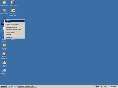
49. Select “Map Network Drive”
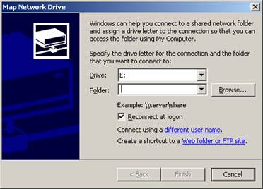
50. In the “Folder” blank, enter the following:
“\\129.252.25.35\pcm” and hit return.
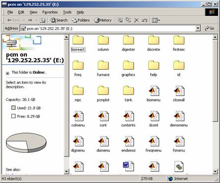
This mounts a network folder onto your local PC, giving you access to
the PCM Matlab files.
You should get the following window:
51. Note the letter of the drive. In this case, the drive is mapped as “E:”
52. Close the window and start MATLAB.
53. You should get the following PC Matlab
window:
54. At the command prompt in the “Command Window” enter
the following:
>> cd e:
(“e:” is the mapped drive letter.)
55. At the command prompt in the “Command Window” enter
the following to start the Process Control Modules:
>> mainmenu
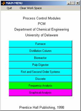
56. From the buttons on the mainmenu
screen, push the button for the Furnace:
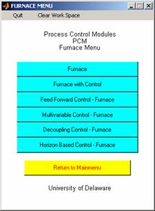
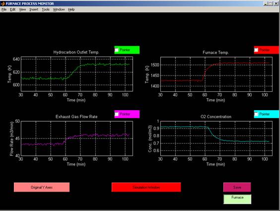
57. From the furnace menu, select “Furnace” to start the
open loop simulation:
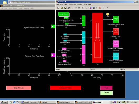
58. Note that there are two windows, a “Process Monitor
Window” and the “Furnace” simulation window.
Try quickly switching between the two windows using the “Process
Monitor” button in the furnace window and the “Simulation Window” button in the
Furnace Process Monitor window.
59. To start the simulation, in the Furnace window, hit
the “play” button in the top, second from the right:
60. Alternatively, you could select from the “Simulation”
menu the “start” option. Alternatively,
you could hit Control-t to start the simulation.
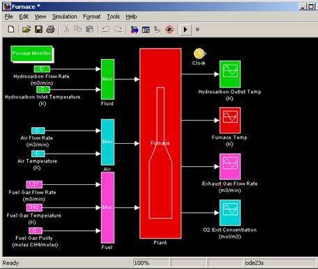
61. The simulation should start to run, simulating a
heated tube furnace:
62. In the Furnace window, double click on the “Fuel Gas
Flow Rate” button in the lower left section of the simulation.
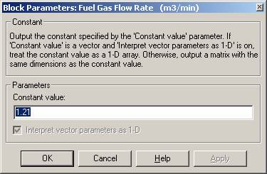
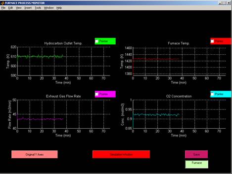
63. Change the value from 1.21 to 1.31 and then hit “ok”,
then quickly double click on the “Process Monitor” button in the upper left
corner of the furnace window. You should
see a dynamic change in the process measurements.
64. Try making other small changes in parameters and
examine the changes in the furnace measurements.
65. Print out a copy of the Process Monitor, with your
name on it, that shows at least one dynamic transient in the furnace system.
DIFFERENTIAL EQUATION EDITOR TUTORIAL
66. Close all PCM windows.
67. At the Matlab command
prompt, type:
>> dee
The following window will appear.
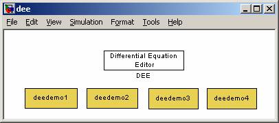
68. Double-click on “deedemo1”. This loads the Van der
Pol Equation demo.
The Van der Pol
equation is a second-order nonlinear ODE of the form:![]()
As with all higher-order ODEs, it can be decomposed
into a system of first-order ODEs. When m is large (~1000),
the system becomes stiff, so this equation becomes a good system to test the
stiff-solving capabilities of an integrator.
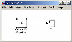
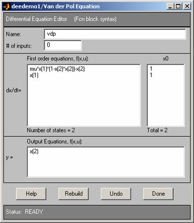
69. Double-click on the “vdp”
block. This brings up the differential
equation editor window:
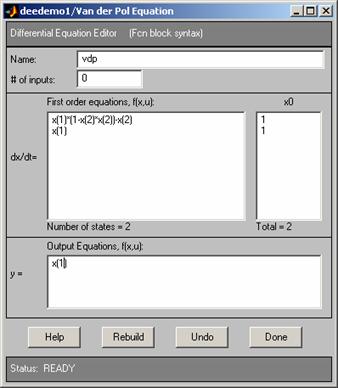
70. To study this system properly, it is necessary to
change some of the default properties.
The demo has done most of the work for decomposing the second-order
system into two first-order systems, but m was left implicitly
as 1. To add an adjustable m, multiply the first term in the first “dx/dt=”
equation by “mu”.
Also, the output (“y”) of interest is really x and not dx/dt, so change the output equation in “y=” to “x(2)”. Check your
work with the figure below to make sure it is correct. Click “Done” when you are finished.
71. In the command window, type:
>> mu = 1;
This tells the Differential Equation Editor what value to use for “mu”.
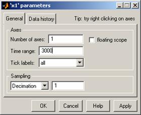
72. It is also necessary to change some of the default
plotting properties. Select the scope
window that was opened when you opened the demo:
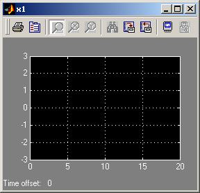
Select the “Parameters” button. (To the
right of the printer.) This brings up
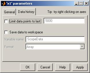
the Parameters window:
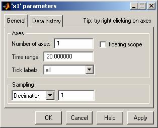
Select the “Data History” tab, and uncheck “Limit data points to last:”. Click “Ok” when you are finished.
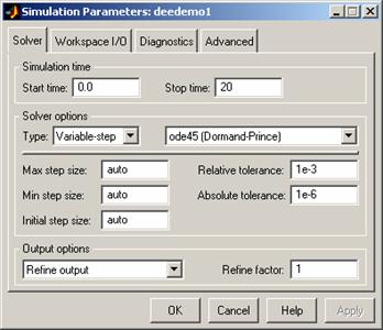
73. Now, from the “Simulation” menu of the deedemo1 sheet,
select the “Simulation parameters” option.
Change the stop time to 20. Click
“Ok” when you are done.
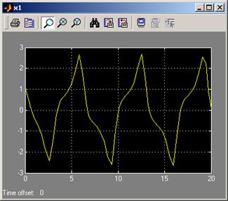
74. Again from the “Simulation” menu, select “Start”. You should see the solution plotted in the
scope. This non-stiff case completes
rapidly.
75. Now it is time to examine the system when the
equations are stiff. In the command
window, type:
>> mu = 1000;
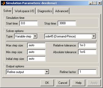
In the scope’s “Parameters” window, select the “General” tab and set “
In the “deedemo1” window, select the “Simulation” window and “Simulation
Parameters”. Change “Stop Time” to 3000.
76. Run the simulation again using the “Simulation” menu
and the “Start” option. You will see the
scope progressing very slowly. If you do
not wish to wait, you can stop the simulation before it finishes. (Make sure you run at least to t = 1000.)
77. The slow performance occurred, because Simulink’s default solver does not handle stiff systems
very well. If you know you are working
with a stiff system, you can change Matlab’s solver
to one that is designed to handle it. In
the “Simulation” menu, select “Simulation Parameters”. Under “Solver Options”, change ode45 to
ode23s. Click “Ok” when you are
finished.
78. Run the simulation again (“Simulation” ->
“Start”). You should see in the scope
that it completes the simulation almost instantly.
79. As you have just seen, the differential equation
editor is a simple way to add systems of ODEs to a Simulink worksheet.
It lets you easily change different parameters of the system and observe
how the output changes. Feel free to
experiment further with the Van der Pol system or any of the other Differential Equation Editor
demos.